Principal Component Analysis (PCA)

Principal component analysis (PCA) is a dimensionality reduction method that transforms a large set of variables into a smaller one but still containing most of the information in the large set.

BESH Stat add-in starting from version 0.22 offers a new Multivariate analysis menu (multivariate refers to the analysis with more than one dependent variable (outcome) and multiple independent variables; in contrast to multivariable models that are used for the analysis with one outcome and multiple independent variables). BESH Stat currently contains the first multivariate method – Principal Component Analysis. Future releases will add new methods including Factor Analysis, Correspondence analysis, Discriminant analysis etc. Version 0.22 adds also 3D scatter plot and Scatterplot Matrix, both of them can help with multidimensional data exploration.

Example

Let’s use the protein data. The protein data set is a real-valued multivariate data set describing the average protein consumption by citizens of 25 European countries. For each country, there are nine columns, corresponding to the different types of proteins. I used first three variables (Read Meat, White Mean, and Eggs) in the 3D scatter plot example in previous post.

Explore input variables

Now we going to explore all variables in the scatter plot matrix first. Download BESH Stat version 0.22 or later, install it. Then open protein.csv file go to add-ins tab, click on BESH Stat → Graphics → Scatterplot Matrix. PCA only works with numerical continuous variables so country variable from the dataset is not used. Notice the correlation between input variables and check the scatter plot matrix of all nine principal components later in the text having all correlation coefficient equal to zero.

Scatter Plot Matrix of Protein Data. Lines on the charts represent simple linear regression fit. Pearson correlation coefficient values are printed on the upper-left section of the plot and corresponding two sided p-values on the lower-right section of the plot.

Conducting PCA

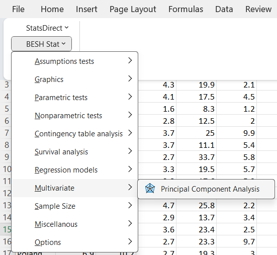
Open protein.csv file sheet and go to add-ins tab, click on BESH Stat → Multivariate → Principal Component Analysis.

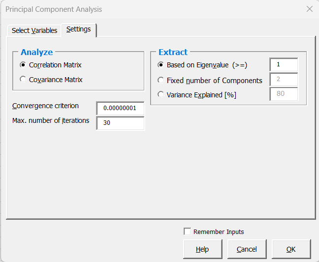
How to run Principal Component Analysis (PCA) in BESH stat add-in.

On the Select Variables tab select all variables and on Settings tab use options as on the screenshot below.

Run PCA on all numerical variables from the protein dataset.

BESH Stats performs following steps to create PCA outputs:

Standardize the range of continuous initial variables (when Correlation matrix is selected. This should be used as a default otherwise units of measurements of individual variables if not identical will influence the results.). Standardization is computed for each variable as z = (value – mean)/standard deviation.
Compute the covariance matrix of the standardized (or centered) variables. Note: covariance matrix of standardized variables is identical to the correlation matrix. .
Compute the eigenvectors and eigenvalues of the covariance matrix to identify the principal components. BESH Stat provides covariance/correlation matrix, eigenvectors, eigenvalues on the PCA results sheet.
Create a loadings vector to decide which principal components to keep. We selected option to extract number of components based on the Eigenvalue > 1. This is otherwise called as a Kaiser rule. BESH Stat provides variable explained by each principal component, and selected component loadings on the PCA results sheet. Note: Component loadings are identical to the Eigenvectors but sign is adjusted based on the sign of the highest (in absolute value) eigenvector value to help the interpretation of principal components.
Recast the data along the principal components axes. BESH Stat provides the reduced data (estimate of each observation in the dataset) on the Data sheet as “Reduced_Data_PC1”, “Reduced_Data_PC2”, “Reduced_Data_PC2” variables, because 3 components were extracted based on the Kaiser rule.

Results

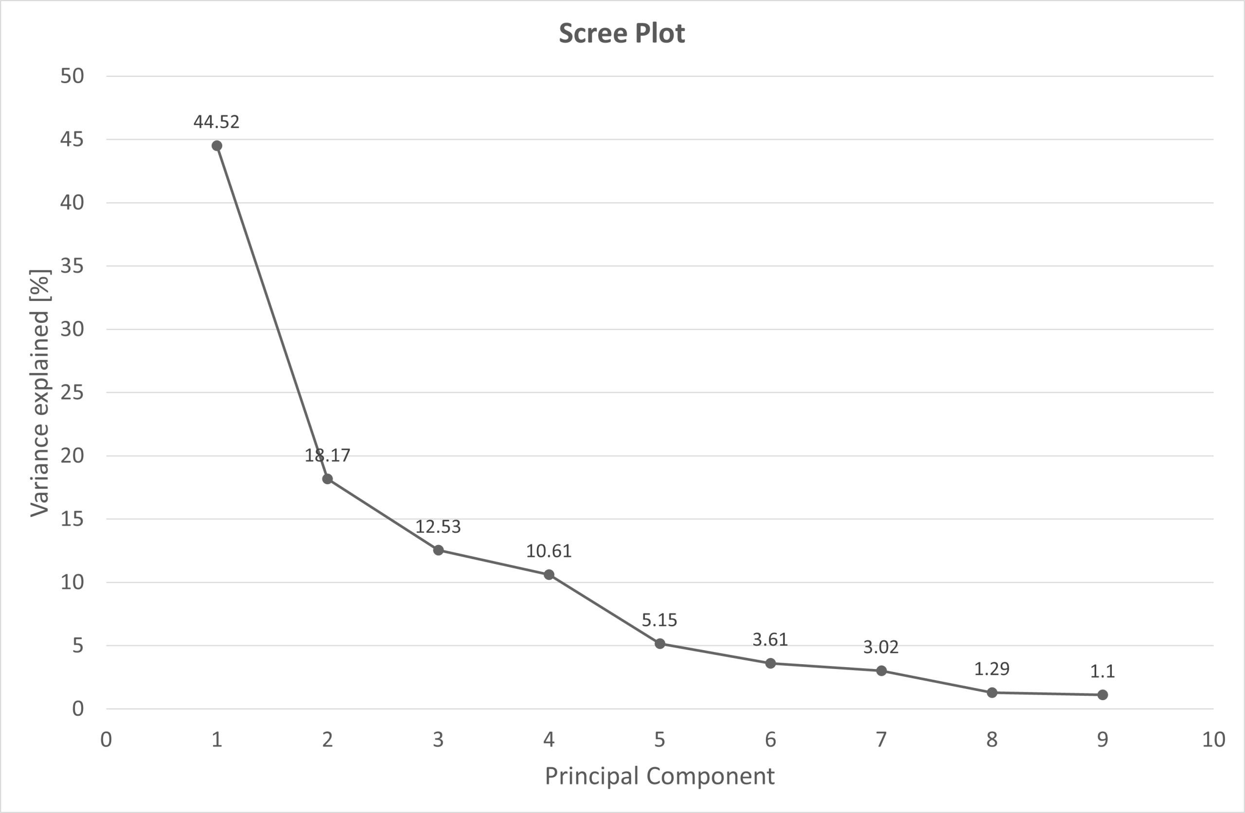
Scree plot display principal components against the percent of variance explained by principal component, it can be used to determine the number of principal components to retain.

Scree Plot of principal components computed on the Protein data.

Score plot, Loading plot, Biplot

Another standard graphical representation of principal components is using the loadings plot, score plot (or biplot that combines loading plot and score plot into a single chart). BESH stats creates all of them automatically. For interpretation of scores and loadings plot see this.

Symmetric biplot – presenting loadings and scores on one plot. For more discussion on biplot see Data inspection using biplots.

Interpretation of biplot is as follows (taken from SAS help). The cosine of the angle between a vector and an axis indicates the importance of the contribution of the corresponding variable to the principal component. The cosine of the angle between pairs of vectors indicates correlation between the corresponding variables. Highly correlated variables point in similar directions; uncorrelated variables are nearly perpendicular to each other. Points that are close to each other in the biplot represent observations with similar values.

All the variables (loadings represented by blue arrows) that are grouped together are positively correlated to each other, and that is the case for instance for eggs, milk, white meat, and red meat have a positive correlation to each other. They are also strongly and positively correlated with the first principal component. The longest the arrow is the better that variable is represented with first two principal components.

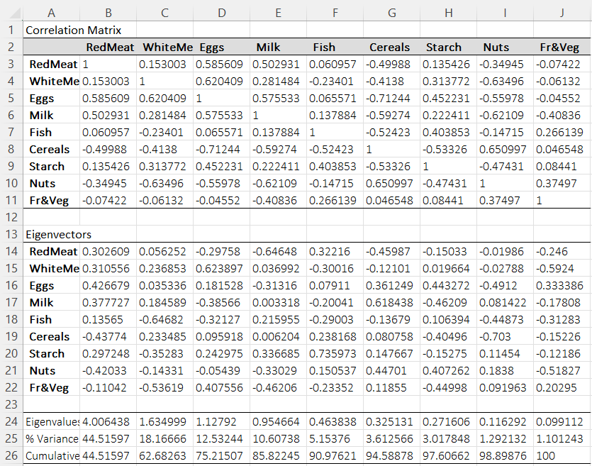
BESH stat output – Correlation Matrix, Eigenvectors, Eigenvalues

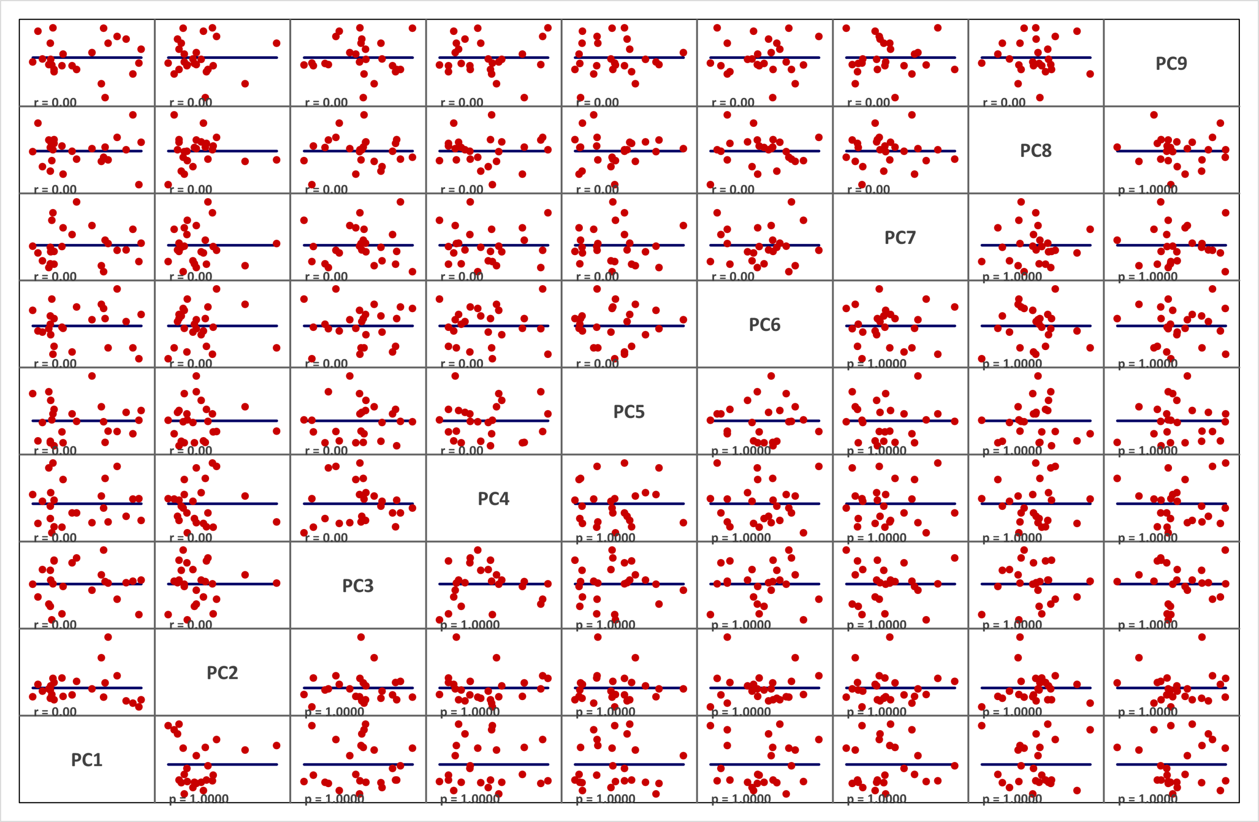
PCA results, correlation matrix of input variables, eigenvectors, eigenvalues, % of variances explained.

Principal components are uncorrelated

If we run the PCA using the Extract option as variance explained [%]= 100 or Fixed number of components = 9 (equal to number of input variables.) and plot the scatter plot matrix of extracted components (Reduced_Data_PCx columns from the BESH stat output in the Data sheet. They are renamed on the scatter plot matrix below to PCx to nicely fit on the available space) we will get the following chart. We can see that components are orthogonal (un-correlated).

Scatter Plot Matrix of all nine principal components created from the Protein data. Notice that all components are uncorrelated to each other, because principal components are computed in such a way to be uncorrelated.