
One-Way ANOVA is used to determine whether there are statistically significant differences between the means of three or more independent (unrelated) groups.
Assumptions:
- Independence of observations
- Normally distributed groups
- Homogeneity of variances (similar variance spread among groups)
One-way ANOVA tests the Null hypothesis that All group means are equal against the alternative hypothesis that At least one group mean is different.
Example
Consider a fictious clinical research study with objective to compare the effectiveness of three different antihypertensive drugs (Drug A, Drug B, Drug C) in lowering systolic blood pressure after 8 weeks of treatment.
Sample Data (Systolic BP Reduction in mmHg):
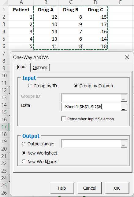
| Drug A | Drug B | Drug C |
| 12 | 8 | 15 |
| 10 | 9 | 17 |
| 14 | 7 | 16 |
| 13 | 6 | 14 |
| 11 | 6 | 18 |
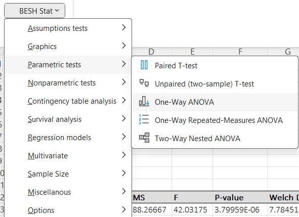
To perform One-Way ANOVE using BESH Stat select excel addin tab and from the BESH stat excel addin menu select Parametric tests → One-Way ANOVA.
But before doing that we should first explore the data and test the ANOVA assumptions. From BESH stat excel add-in menu select Graphics → Box and Whiskers
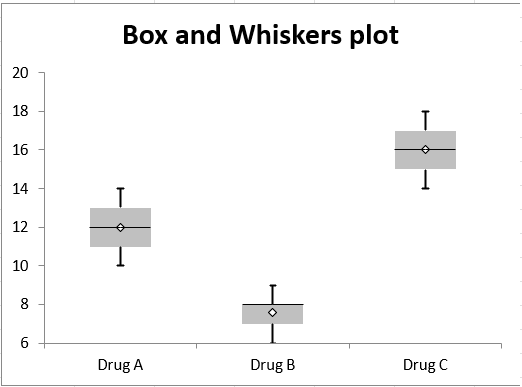
Already from the chart we can see the differences in the BP changes between treatment groups where Drug C caused the largest BP change (mean change equal to 16 mmHg) and Drug B the smallest change (mean change equal to 7.6 mmHg). To compute descriptive statistics elect Assumptions → Descriptive statistics from BESH stat excel add-in menu.
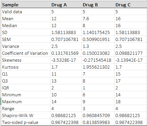
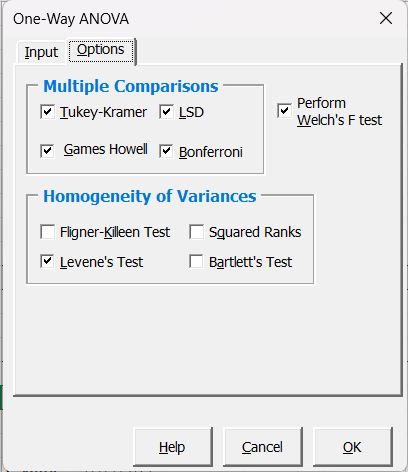
BESH stat also have capabilities to test the ANOVA model assumptions. The independence of observations is given by the study design. To test normality assumption we you can either select Assumptions test → Normality Tests or alternatively when computing descriptive statistics check the Shapiro-Wilk test option. Shapiro-Wilk test for all three groups is non-significant and also from the box plot we see that data are symmetrical with mean ≈ median and skewness ≈ 0. To test the homogeneity of variance assumption we can either elect Assumptions test → Homogeneity of variance or alternatively we can check the Levene’s test from on the One-way ANOVA userform options tab (see screenshot below). Levene’s test p = 0.69 (see screenshot below) is non-significant so we can assume homogeneity of variation (if violated BESH stat can compute Welsch’s F-test that takes into account un-equal variances.)
ANOVA table
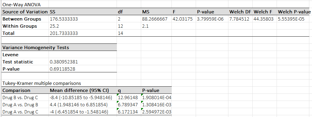
From the table we see p < 0.0001 so we can reject null hypothesis and conclude that at least one group mean is different.
Conclusion: There is a statistically significant difference in systolic blood pressure reduction among the three drugs.
To find out which groups differs we can perform post-hoc multiple comparisons test procedure. BESH stat offers Tukey-Kramer HSD, Games-Howell, Fisher’s Least Significant Difference (LSD), and Bonferroni. We will use Tukey-Kramer HSD as it controls the overall alpha level when performing all pairwise comparisons, allow us to compute simultaneous confidence interval and has a high power.
From the output we can see that all groups significant differs from one another (all p < 0.01).